*Note: IDRISI commands are specified as follows:

Commands:  COMMAND 1 – COMMAND 2 – ETC.

This format applies to all remaining laboratory assignments.

(If you would like more detail on any commands or functions, refer to the ‘Help’ index in IDRISI)

Preprocessing encompasses a variety of operations designed to make a set of image bands more manageable, informative and accurate. Processes usually fall into one of the following categories:

·        Creating Image Subsets

·        Feature Extraction

·        Radiometric Correction

·        Geometric Correction

Each of these steps is well documented in Campbell’s chapter 10; Jensen chapters 6 and 7. The purpose of this exercise is to introduce two aspects of preprocessing - creating “subsets” and “feature extraction” - and to apply these techniques to the 1986 LANDSAT 5 MSS (Multi-Spectral Scanner) image of Mexico’s Sierra Basin, a volcanic plateau about 150km southeast of Guadalajara.

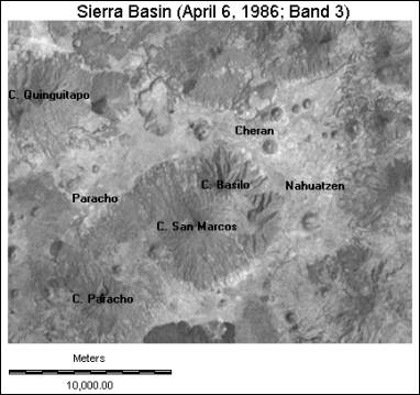
Figure 1: The study site.  

Step 1 - Creating Image Subsets (Campbell pages 290 - 292)

The study area you have been assigned is depicted in Figure 1. This region of basin contains the towns of Paracho, Cheran and Nahuatzen, as well as the surrounding volcanic peaks, the largest of which is Cerro de Paracho. Your objective is to develop a land cover inventory of the area, including forested land, urban areas and agricultural regions.

The original LANDSAT image covers a much greater spatial extent than the study area. By reducing the image such that it contains only the data regarding the specified area – create a “subset” – the complexity of analysis will be reduced, storage requirements and processing times will be limited, and results will likely be easier to interpret and verify.

Before proceeding, make sure that you have copies of the original MSS bands in your Lab #5 directory (each image has a .rst and .rdc file):

Band 1 (0.5 - 0.6 micrometers, visible green     )
Band 2 (0.6 - 0.7 micrometers, visible red        )
Band 3 (0.7 - 0.8 micrometers, near infrared    )
Band 4 (0.8 - 1.1 micrometers, near infrared   )  

Display the Band 3 image with the Grey Scale palette with the “Autoscale” option and no “Title”. Compare the extent of this image to the study area pictured in Figure 1.

The original image data used in this exercise is actually a subset of an April 20, 1986, LANDSAT 5 MSS image. The full image represents a 185 X 185-kilometer swath – roughly 35,000 square kilometers in area. (The original 90-meter resolution has also been re-sampled to 60-meters for topographic correction and registration purposes.)

Step 1:  Creating image subsets

1.      Set the Project Environment to the directory containing the Lab 5 folder.

2.      Commands:  REFORMAT – WINDOW

3.      Set number of files to 4.

4.      Select the each of the four input images by clicking the browse icon.

5.      In “Output prefix” Select an appropriate prefix ( refor ) for output files to create a unique identifier.  Click on “add prefix to file name”

6.      In “Window specified by” select geographical positions option.  This option allows the user to enter minimum/maximum UTM coordinates (in meters) of the subset image.

7.      Enter the UTM positions, as specified in the Table 1, in the appropriate box.

8.      Leave other settings as default.

9.      Select OK to process the images.

                    TABLE 1: Subset Image Coordinates

The result should be a set of four images - MSS Bands 1 through 4 - that now contain only the area selected as the study site. Display the new Band 3 image using the Grey Scale palette and “Autoscale.” It should look similar to Figure 1.

Take a few minutes and zoom in on Figure 1 to find the area that is located.

Questions:

1)      The METADATA command [Commands: FILE - METADATA] provides information on the projection, file structure, size, and resolution of an image. Compare the metadata of the original image to that of the subset image - what has changed?

2)      How many pixels make up the original image and the subset image? Show your work.

3)      What is the approximate area of the subset image, to the nearest square kilometer? Show your work.

4)      Display the Band 3 subset image. Examine the image’s histogram. Why does “autoscale” produce a good result?  

Step 2:  Feature Extraction (Principal Components Analysis) (Campbell pages 287 – 291; Jensen pages 172-179)

When working with large multi-band imagery data it is often necessary to reduce the volume of data to only that which is deemed essential for image analysis. Frequently, different bands of multi-image data contain similar information. Figure 2 illustrates this point. In a highly vegetated area, for example, the use of both a blue visible and red visible band would most likely be redundant. Vegetation responds similarly in both of these wavelengths. By removing one of these bands, the volume of image data is reduced dramatically, yet the amount of unique information lost may be statistically negligible.

Figure 2: Typical spectral reflectance of vegetation

In a previous exercise, we examined which bands were highly correlated and eliminated those redundant ones.  If you remember, however, the correlations between the bands was not perfect and we perhaps lost some information.  Is there a better way is reduce the data volume (number of bands) we have to examine, yet maintain the greatest amount of information. 

Principal Component Analysis (PCA) is a mathematical process that can be used to transform a set of image bands into a new set of virtual bands (called components) where correlation between the components is minimized. Therefore, each component contains information different from the others. Each component is a statistical description of the variability present in all bands, and they are ordered in terms of the amount of variability they explain. “Component 1” represents the optimum combination of bands and accounts for the greatest variability in brightness in the image, “Component 2” the second-most, and so on. This new data can then be correlated with the original image data to identify the combination of original bands that contain most of the unique information.

What is the relation between the spectral bands and the components?  The answer is determined from the “loading”, or how each component correlates with each band.  From a table of load values one can determine the relative influence of each band on each component.  Jensen includes a good description of this.

Although this exercise uses a relatively small data set, this is an important and often used technique in analysis of remotely sensed information. Therefore, we will perform a basic PCA on the study area image created in Step 1 to determine which original bands contain the most information.  [N.B. All subsequent exercises will use the study-area images (subset images) created in Step 1.]  The results will be used in future classification exercises.

1.      Set the Project Environment to the directory containing the Lab 5 folder.

2.      Command: ANALYSIS - IMAGE PROCESSING - TRANSFORMATION – PCA

3.      Select “Calculate covariances directly” option.

4.      Set number of files to 4.

5.      Add the reformated image bands by clicking the browse icon for each line.

6.      Select 4 components to be extracted.  It is general practice to extract as many components as there are bands. 

7.      Enter a prefix, pca, for the output data

8.      Select the “Unstandardized variables” option. 

[A discussion of covariance calculation and the difference between using unstandardized/standardized variables is beyond the scope of this exercise. The default settings used by IDRISI are the most commonly used approach. ]

9.      Click OK to process.

The results will automatically appear on the screen. The structure of this data is explained as follows:

VAR/COV -          The variance/covariance matrix. This information is used by the PCA algorithm to construct the components

COR MATRX -     The correlation matrix. This is the correlation between bands. Bands that are highly correlated represent much of the same information (a value of 1 represents perfect correlation, a value of 0 no correlation.)

COMPONENT -  This is the component summary table. The Eigenvalues express the amount of total variance in all four image bands explained by each component; these values are also expressed as a percent of total variance (% VAR.). (The Eigenvectors are used by the transformation equation; for the purposes of this exercise, they can be ignored.).

LOADING -         The loadings matrix. The Loadings refers to the degree of correlation between the original bands with the components. The band correlating most highly with (and therefore most similar to) component 1 contains the most information relative to the other original bands. The band correlating most highly with component 2 is the second-most informative, and so on.

Save a copy of this table as a textfile; it will be useful in later exercises.
 

Questions:

Refer to the Correlation Matrix:

10)  Why is the diagonal equal to 1.0?

11)  Would you use both Bands 1 and 2 in subsequent analysis? Why or why not? (Describe the relationship between these bands.)

12)  Explain one scenario in which your answer to #11 might be different? (Hint: Think about the spectral response of surface features to the four MSS wavelengths.)

Refer to the Component Matrix:

13)  Examine the “% var.” (percent variance) for each of the components.  What do they mean?

14)  How much of the variance is explained by the first two components?  Show your work.

15)  How much variance do the final two components explain?  Show your work.  

At this point, it might be useful to display the 4 PCA component images using the Grey Scale palette and autoscale

16)  For further analysis, what components would you use and which would you discard?  Explain your answers.  Refer to the histograms for each component image to help you answer this question. What does Component 4 most likely represent?

17)  What percentage of data would you be discarding?

Refer to the Loadings Matrix:

18)  What original band image(s) most resembles Component 1?  Discuss.

19)  What original band image(s) most resembles Component 2?  Discuss.

20)  What original band image(s) most resembles Component 3 and 4? Discuss

21)  Which three original bands contain the most information regarding the study site? Given their correlation, and the loading, did you learn anything from the PCA analysis that you otherwise might not have done if you were going to select the manually for analysis?

Refer to LAB #4:

22)  Assume that you can only use two of the three SPOT image bands (pdxspotm) for image classification. Which bands would you use?

23)  How much information would you be retaining if you used the first two components for subsequent analysis?

24)  Explain some of the problems with using the mathematically derived components for image analysis rather than the original bands. What are the benefits to this type of approach?  

25)  What are the drawbacks? (HINT: What do you know about the original image bands that you do not about the components?)